Fit quadratic-plateau models in R

How does one fit and plot a quadratic-plateau model in R?

Like this:

quad_plateau(data)

Or at least that is how it works once I explain a few things. Like my post on linear plateau models in R, this post is for the person¹ who has been googling how to fit quadratic plateau models in R. This post provides three ways to accomplish this, and also shows off my convoluted creative function that helps one do quadratic plateau fits and make a ggplot style figure all at once. I’ve written this post in the context of soil test correlation, so the code isn’t an out-of-the-box solution for any kind of analysis.

¹ Probably a grad student

To make your life easier, here is a link to my R code so that you do not have to copy and paste code chunks from this page. Note my R programming language has a heavy tidyverse accent.

So first, get out your library card and borrow some packages.

library(agridat)   # for the data
library(tidyverse) # for data manipulation and plotting and so on
library(nlraa)     # for self-starting models
library(minpack.lm)# for nls with Levenberg-Marquardt algorithm
library(nlstools)  # for residual plots
library(modelr)    # for the r-squared and rmse
library(devtools)  # for sourcing the quad_plateau() function in Method 3

The Data

The data is suppose to be some cotton trials based on Cate and Nelson (1971), and can be accessed through the agridat package. Basically, more potassium measured in the soil should correlate to more cotton yield, but the relationship will most likely not be linear. Fitting a model to determine something about this relationship is central to the soil test correlation process. Let’s plot it to see what we’re working with.

cotton <- tibble(x = agridat::cate.potassium$potassium,
                 y = agridat::cate.potassium$yield)

cotton %>% 
  ggplot(aes(x, y)) +
  geom_point(size = 2, alpha = 0.5) +
  geom_rug(alpha = 0.5, length = unit(2, "pt")) +
  scale_x_continuous(breaks = seq(0, 1000, 20)) +
  scale_y_continuous(limits = c(0, 110),
                     breaks = seq(0, max(cotton$y) * 2, 10)) +
  labs(title = paste(
    "Relative yield and soil potassium for", nrow(cotton), "cotton trials"),
    y = "Relative yield (%)",
    x = "Soil Test K (mg/kg)")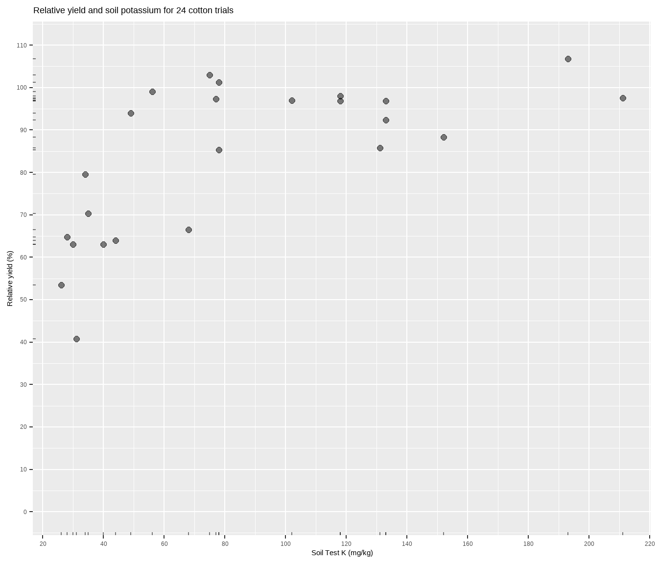

The relationship between soil test potassium (STK) and relative cotton yield may be nonlinear². Perhaps a polynomial function could be fit, or the data could be transformed, but we’ll fit a nonlinear model known as the quadratic-plateau (QP), or quad-plat³. The QP model is a type of segmented model, and QP is nice in that it has a curved component (important to biological systems) that meets a zero-slope plateau at the join point (important for researchers). Looking at the plot, notice how the relative yield of the cotton does not appear to increase anymore from about 70 to 200 mg kg^-1 K (the plateau!). Scroll to the bottom of this page if you struggle to visualize this.

² No one will judge you if you hold a clear, plastic ruler up to your computer screen.

³ This isn’t true, but I wish it was.

The QP Function

The equation for the QP is a quadratic up until the join point: y = a + bx + cx². While we could define the QP equation inside the nls() function later, let’s make a separate function.

# a = intercept
# b = slope
# c = quadratic term (curvy bit)
# jp = join point = break point = critical concentration

qp <- function(x, a, b, jp) {
    c <- -0.5 * b / jp
    if_else(condition = x < jp,
            true  = a + (b * x) + (c * x * x),
            false = a + (b * jp) + (c * jp * jp))
}

This function says that up until the join point, the relationship is a second-order polynomial (quadratic), after which it hits a flat line (plateau). This model is sometimes also called quadratic-plus-plateau. That join point is important. In the context of soil fertility, it represents a critical soil test concentration for the nutrient of interest. The join point of a “quad-plat” will always be higher than with a linear plateau, an important consideration for another time and place.

The qp function will be used inside the base R nls() function inside my quad_plateau() function later. So look for them there.

Method 1: base R

Using the nls() function in base R requires that we provide the formula (in this case the QP function), the data, and starting values. Starting values are critical⁴, and the computer doesn’t really know where to start, so poor starting values may result in failures of the model to converge as the algorithms working their tails off behind the scenes try to home in on the best values. It helps, though, to keep in mind that with this sort of data we can expect:

⁴ What if the starting values result in a failure of converge? Check out these tips from Dr. Miguez.

1. the intercept will not be greater than the maximum Y value
2. the slope will be positive (the quadratic term must therefore be negative)
3. the join point cannot not be less than your minimum X value (and, ideally, will be less than than your maximum⁵).

⁵ If the join point is equal to or greater than your maximum X value, then you have not fitted a QP model. You have fitted a regular, ol’ fashioned quadratic.

Pro-tip: the lower and upper arguments can be used inside nls() to set parameter limits.

Get starting values guessing

Eyeballing that scatter plot, I’m trying to visualize in my mind’s eye a quadratic line coming up and bending over at a join point. The join point is easiest to imagine, and I’d guess it’s somewhere between 60 and 80 ppm K⁶. Going to the left, that imaginary quadratic line looks like it might intercept the Y-axis around 0. The slope of that line would be positive, and looks like maybe it’s around 2 (2% RY gain for every 1 ppm increase).

⁶ Experiment by adjusting the starting values and seeing if you get the same model. By setting `jp = 20` I got an error as the convergence failed.

fit1 <- nls(formula = y ~ qp(x, a, b, jp),
            data = cotton,
            start = list(a = 0, b = 2, jp = 70))

summary(fit1)

Formula: y ~ qp(x, a, b, jp)

Parameters:
   Estimate Std. Error t value Pr(>|t|)    
a   12.8637    22.9922   0.559 0.581752    
b    1.9124     0.9076   2.107 0.047291 *  
jp  86.1973    19.5721   4.404 0.000247 ***
---
Signif. codes:  0 '***' 0.001 '**' 0.01 '*' 0.05 '.' 0.1 ' ' 1

Residual standard error: 10.83 on 21 degrees of freedom

Number of iterations to convergence: 6 
Achieved convergence tolerance: 4.205e-06

And it worked! The response curve is 12.8 + 1.91x - ??x² up to 86 ppm K.

Wait, what is the quadratic term? It’s not explicitly in this model, but it is in the QP formula which is c = -0.5 * b / jp, or -0.011.

Get starting values with augmented guessing

If you struggle to visualize in your mind’s eye the curve going through the points, then another way to estimate starting values is to mess around with sliders on a graphing calculator like Desmos. In our case, enter the equation a + bx - cx², set the value ranges for the parameters, and move the sliders and their value ranges until you get something you could imagine would go through your points. Zoom out until the X-axis and Y-axis ranges match your dataset, then move sliders, then use those values in the starting values list like before. The starting values don’t have to be spot on, just close enough.

Get starting values by fitting a quadratic polynomial

If you’re a sane person, you might decide to make math get the starting values for you by fitting a regular ol’ quadratic polynomial⁷. From this the intercept and slope can be estimated more precisely, and the join point can then be estimated by taking the median of the soil test values.

⁷ Also known as a quadrapoly.

quadratic <- lm(y ~ poly(x, 2, raw = TRUE), data = cotton)

start_values <- coef(quadratic)

start_values

            (Intercept) poly(x, 2, raw = TRUE)1 poly(x, 2, raw = TRUE)2 
           45.227449132             0.727177376            -0.002363206 

fit2 <- nls(formula = y ~ qp(x, a, b, jp),
            data = cotton,
            start = list(a = start_values[1],
                         b = start_values[2],
                         jp = median(cotton$x)))

summary(fit2)

Formula: y ~ qp(x, a, b, jp)

Parameters:
   Estimate Std. Error t value Pr(>|t|)    
a   12.8650    22.9913   0.560 0.581698    
b    1.9124     0.9075   2.107 0.047287 *  
jp  86.1986    19.5723   4.404 0.000247 ***
---
Signif. codes:  0 '***' 0.001 '**' 0.01 '*' 0.05 '.' 0.1 ' ' 1

Residual standard error: 10.83 on 21 degrees of freedom

Number of iterations to convergence: 6 
Achieved convergence tolerance: 8.333e-06

It worked again, even though the starting values weren’t super close to the final parameter values.

Method 2: nlraa

Better than providing starting values to nls is to use a function that can “self-start”. The nlraa package provides just that, self-starting functions for a quadratic plateau model. There are three functions available, but the one with 4 parameters seems to have issues. The SSquadp3 function is parameterized for the quadratic term, but since I’m more interested in the join point, let’s use the SSquadp3xs function⁸.

⁸ the author uses xs as the critical x-value or break-point whereas I’ve chosen jp to represent the “join-point”

fit3 <- nls(formula = y ~ SSquadp3xs(x, a, b, jp),
            data = cotton)

summary(fit3)

Formula: y ~ SSquadp3xs(x, a, b, jp)

Parameters:
   Estimate Std. Error t value Pr(>|t|)    
a   12.8640    22.9920   0.559 0.581741    
b    1.9124     0.9075   2.107 0.047290 *  
jp  86.1976    19.5721   4.404 0.000247 ***
---
Signif. codes:  0 '***' 0.001 '**' 0.01 '*' 0.05 '.' 0.1 ' ' 1

Residual standard error: 10.83 on 21 degrees of freedom

Number of iterations to convergence: 7 
Achieved convergence tolerance: 1.586e-06

Flawless.

Method 3: Convoluted way

My custom, wrapper-style function quad_plateau()⁹ fits a QP model and either gets useful numbers into a table or plots it visually. Getting results into a table means that this function is compatible with tidyverse/tidymodels style work, usable on grouped data frames and so on. Getting results into a plot could be done with a separate function, but why not cram it all into one? Here are the steps of the function:

⁹ I’m not a function wizard, but I’m trying, so forgive any poor coding practices.

1. Run nls()¹⁰ with the SSquadp3xs function. Try nlsLM if nls fails.

2. Test goodness-of-fit with AIC, RMSE, and R².

3. Get model coefficients for response curve equation.

   1. It would be nice to get a confidence interval for the join point (critical soil test value), but this requires bootstrapping which I won’t do here for now.

   2. Optional: look at standard error and p-values for the coefficients, though these may not matter much.

   3. Optional: get the soil test value at some point below the join-point, such as 95% of the maximum yield plateau. This is reported in the adjusted_cstv column.

4. Create a table of results.

   OR

5. Plot the cotton yield data with a regression line using nls and the model final values as starting values (which should ensure identical results).

   • There are arguments for making residual plots as well, and for adding a confidence band to the fitted line in the plot. These are false by default.

¹⁰ minpack.lm::nlsLM() can sometimes find a solution and converge where the base R nls() cannot, probably due to using a different algorithm (Levenberg-Marquardt). But you can test whether these two functions reach the same final results for your data.

devtools::source_url("https://raw.githubusercontent.com/austinwpearce/SoilTestCocaCola/main/quad_plateau.R")

# run `quad_plateau` without parentheses in R console to see source code

Convoluted result

So how do you fit a quadratic plateau model in R? Like so:

quad_plateau(cotton, x, y)

# A tibble: 1 × 12
  intercept slope   curve equation       cstv plateau   AIC  AICc  rmse rsquared
      <dbl> <dbl>   <dbl> <chr>         <dbl>   <dbl> <dbl> <dbl> <dbl>    <dbl>
1      12.9  1.91 -0.0111 12.9 + 1.91x…    86    95.3   187   189  10.1     0.68
# ℹ 2 more variables: cstv_pom <dbl>, percent_of_max <dbl>

The model is written out in a data frame, ready for other use and manipulation. Having it in a tibble is really helpful if for example you have a grouped data frame of different fertilizer trials, and want to perform a QP fit to each group using something like group_modify().

If you want to plot it along with an overlay of model results, use the plot = TRUE argument and add your labels. Use group_map() if you want to “loop” this over multiple groups in your data frame.

quad_plateau(cotton, x, y, plot = TRUE)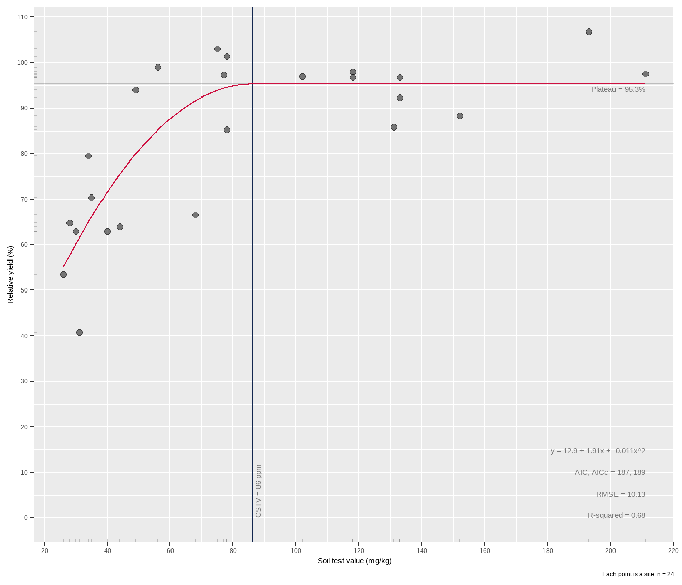

The critical soil test value for potassium appears to be around 86 mg kg^-1 K, higher than the linear plateau model. In the case of this dataset, the wide confidence band probably has to do with data availability. There are gaps in the data, including a hole between 40-80 ppm STK and 65-90% RY. Basically the model lacks confidence in the fit approaching the join point, and this is reflected in the wide gray RY confidence band shown around the red line in the plot. The experimenter needs more data in that gap.

Now, what if the two points with “high” STK (> 180 ppm), were removed? How would that change the analysis? Go back and test yourself¹¹. How do other models compare? Linear plateau? Mitscherlich? Cate-Nelson?

¹¹ Hint: filter()

More packages related to nonlinear functions in R

• nlraa package by Fernando Miguez (highly recommend)

  • he also has a series of YouTube videos worth checking out.

• rcompanion package - many examples of models also applicable to agronomy

• nlstools package

• easynls package - it’s quick and dirty, but not as useful as it could be

• nls.multstart package - tries lots of starting values to try and better get at the best values for the equation. But I think for QP models, nlraa package works just fine and using multiple starting values is unnecessary.

Bonus: Quick figure with QP line

What if you just want a quick figure of a QP fitted to your scatter plot points, and do not care so much about the model results and information, etc? Using the self-starting function from nlraa, try the following:

cotton %>% 
  ggplot(aes(x, y)) +
  geom_point(size = 3,
             alpha = 0.5) +
  geom_line(stat="smooth",
            method = "nls",
            formula = y ~ SSquadp3xs(x, a, b, jp),
            se = FALSE,
            color = "#CC0000") +
  labs(title = paste(
    "Soil test correlation with quadratic plateau for", nrow(cotton), "cotton trials"),
    y = "Relative yield (%)",
    x = "Soil Test K (mg/kg)")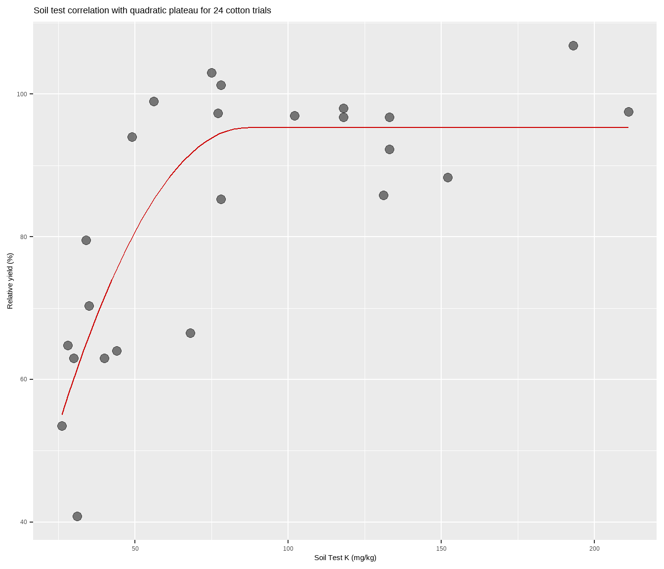

Congratulations! You are now certified to quad-plat in R.