library(agridat)   # for the data
library(tidyverse) # for data manipulation and plotting and so on
library(nlraa)     # for self-starting models
library(minpack.lm)# for nls with Levenberg-Marquardt algorithm
library(nlstools)  # for residual plots
library(modelr)    # for the r-squared and rmse
library(devtools) # for sourcing the lin_plateau() function in Method 3This post is intended for the person1 who has been googling how to fit linear plateau models in R. Like my suspiciously similar post on quadratic plateau models in R This post demonstrates three ways to fit a linear-plateau model, and presents an unnecessary unique function that sort of helps one do linear plateau fits and make a ggplot style figure all at once. I’ve written this post in the context of soil test correlation, so the code isn’t an out-of-the-box solution for any kind of analysis. But you can figure it out.
1 Probably a grad student
So first, load some packages.
The Data
The data is suppose to be some cotton trials based on Cate and Nelson (1971), and can be accessed through the agridat package. Basically, more potassium measured in the soil should correlate to more cotton yield, but the relationship will most likely not be linear. Fitting a model to determine something about this relationship is central to the soil-test correlation process. Let’s plot it to see what we’re working with.
cotton <- tibble(x = agridat::cate.potassium$potassium,
                 y = agridat::cate.potassium$yield)

cotton %>%
  ggplot(aes(x, y)) +
  geom_point(size = 2, alpha = 0.5) +
  geom_rug(alpha = 0.5, length = unit(2, "pt")) +
  scale_x_continuous(breaks = seq(0, 1000, 20)) +
  scale_y_continuous(limits = c(0, 110),
                     breaks = seq(0, max(cotton$y) * 2, 10)) +
  labs(title = paste(
    "Relative yield and soil potassium for", nrow(cotton), "cotton trials"),
    y = "Relative yield (%)",
    x = "Soil Test K (mg/kg)")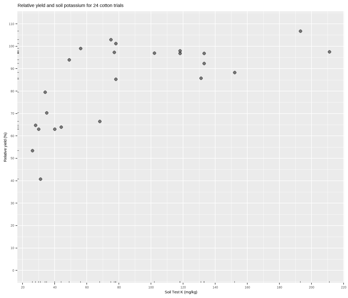
The relationship between soil test potassium (STK) and relative cotton yield may be nonlinear2. Perhaps a polynomial function could be fit, or the data could be transformed, but we’ll fit a nonlinear model known as the linear plateau (LP), or lin-plat3. The LP model is a type of segmented model, and is simpler than quadratic plateaus because there is no curve! Maybe the curve is important to biological systems, but for now note that in a LP model the response line meets a zero-slope plateau at a well-defined join point. Looking at the plot, notice how the relative yield of the cotton does not appear to increase anymore from about 70-200 ppm K (the plateau!). Scroll to the bottom of this page if you struggle to visualize this.
2 No one will judge you if you hold a clear, plastic ruler up to your computer screen.
3 This isn’t true, but I wish it was.
The LP function
The equation for the LP is a line up until the join point: y = a + bx. While we could define the LP equation in the nls() function later, let’s make a function now.
# a = intercept
# b = slope
# jp = join point = break point = critical concentration
#
lp <- function(x, a, b, jp) {
    if_else(
      condition = x < jp,
      true = a + b * x,
      false = a + b * jp)
}
This function says that up until some join point, the relationship is linear, after which the stick breaks and it is a flat line (plateau). Sometimes this model is called broken-stick or linear-plus-plateau. That join point is important. In the context of soil fertility, it represents a critical soil test value for the nutrient in the soil. The join point of a linear plateau will always be lower than with a quadratic plateau, an important consideration for another time and place.
Method 1: base R
Using the nls() function in base R requires that we provide the formula (in this case the LP function), the data, and starting values. Starting values are critical, and the computer doesn’t really know where to start, so poor starting values may result in failures of the model to converge as the algorithms working their tails off behind the scenes try to home in on the best values. It helps, though, to keep in mind that with this sort of data we can expect:
- the intercept will not be greater than the maximum Y value
- the slope will be positive
- the join point will not be less than your minimum X value (and, ideally, will be less than than your maximum4).
4 If the join point is equal to or greater than your maximum X value, then you have not fitted a LP model. You have fitted a regular, ol’ fashioned, straight line.
Pro-tip: the lower and upper arguments can be used inside nls() to set parameter limits.
Get starting values by guessing
Eyeballing that scatter plot, I’m trying to visualize in my mind’s eye a straight line coming up and breaking over at a join point. The join point is easiest to imagine, and I’d guess it’s somewhere between 60 and 80 ppm K. Going to the left, that imaginary line looks like it might intercept the y-axis around 20-30, maybe? The slope of that line would be positive, and looks like maybe it’s around 2-ish (2% RY gain for every 1 ppm increase).
fit <- nls(formula = y ~ lp(x, a, b, jp),
           data = cotton,
           start = list(a = 20,
                        b = 2,
                        jp = 70))
Error in nls(formula = y ~ lp(x, a, b, jp), data = cotton, start = list(a = 20, : step factor 0.000488281 reduced below 'minFactor' of 0.000976562summary(fit)Error in eval(expr, envir, enclos): object 'fit' not foundAnd it failed5. If we try running this again but include trace = TRUE as an additional argument, we see that nls() got close to finishing, but it could be it failed to converge because the data is too noisy/gappy around the values we are guessing the join point.
5 What if the starting values result in a failure of converge? Check out these tips from Dr. Miguez.
Before trying another method to get starting values, let’s try nlsLM() first from the minpack.lm package, which uses a different algorithm.
fit2 <- nlsLM(formula = y ~ lp(x, b0, b1, jp),
      data = cotton,
      start = list(b0 = 20,
                   b1 = 2,
                   jp = 70))

summary(fit2)
Formula: y ~ lp(x, b0, b1, jp)

Parameters:
   Estimate Std. Error t value Pr(>|t|)
b0  39.8156     9.4844   4.198 0.000405 ***
b1   0.7411     0.2077   3.568 0.001814 **
jp  75.0000    10.8416   6.918 7.79e-07 ***
---
Signif. codes:  0 '***' 0.001 '**' 0.01 '*' 0.05 '.' 0.1 ' ' 1

Residual standard error: 11.06 on 21 degrees of freedom

Number of iterations to convergence: 19
Achieved convergence tolerance: 1.49e-08
And it worked! The response equation is y = 39.8 + 0.74x up to 75 ppm K.
Get starting values by fitting a line
If you’re a sane person, you might decide to get starting values for a LP model by fitting a regular ol’ line. From this the intercept and slope can be estimated, and the join point can then be estimated by taking the mean or median of the soil test values. In fact, we could wrap all of these steps into a function.
linear <- lm(y ~ x, data = cotton)

start_values <- coef(linear)

start_values
(Intercept) x
64.2989271 0.2261891 # again, have to use minpack.lm::nlsLM() with this dataset because of noise
fit3 <- nlsLM(
formula = y ~ lp(x, a, b, jp),
data = cotton,
start = list(
a = start_values[1],
b = start_values[2],
jp = median(cotton$x)
)
)
summary(fit3)
Formula: y ~ lp(x, a, b, jp)

Parameters:
              Estimate Std. Error t value Pr(>|t|)
a.(Intercept)  19.2710    14.0272   1.374  0.18398
b.x             1.3325     0.3649   3.652  0.00149 **
jp             56.0000     6.1082   9.168 8.67e-09 ***
---
Signif. codes:  0 '***' 0.001 '**' 0.01 '*' 0.05 '.' 0.1 ' ' 1

Residual standard error: 10.71 on 21 degrees of freedom

Number of iterations to convergence: 15
Achieved convergence tolerance: 1.49e-08
It worked again, but notice that the response equation now is y = 19.3 + 1.33x up to 56 ppm K. Quite a bit different perhaps just by using different starting values. Using a self-starting function that uses an optimization algorithm to get starting values might be a more precise and reliable way to go. Let’s try that.
Method 2: nlraa
Better than providing starting values to nls or nlsLM is to use a function that can “self-start”. The nlraa package provides just that, a self-starting function for a linear-plateau model. For the function SSlinp, the author uses xs as the critical x-value or break-point whereas I’ve chosen jp to represent the “join-point”.
fit4 <- nlsLM(formula = y ~ SSlinp(x, a, b, jp), data = cotton)

summary(fit4)
Formula: y ~ SSlinp(x, a, b, jp)

Parameters:
   Estimate Std. Error t value Pr(>|t|)
a   39.2364    11.2023   3.503  0.00212 **
b    0.7518     0.2668   2.818  0.01030 *
jp  75.0000    13.7752   5.445 2.11e-05 ***
---
Signif. codes:  0 '***' 0.001 '**' 0.01 '*' 0.05 '.' 0.1 ' ' 1

Residual standard error: 11.06 on 21 degrees of freedom

Number of iterations to convergence: 8
Achieved convergence tolerance: 1.49e-08
Flawless (so long as we use nlsLM). This function optimizes the starting values through some sort of searching, and the resulting equation is y = 39.2 + 0.75x up to 75 ppm K, which is similar to the first.
Method 3: Convoluted way
My custom, wrapper-style function lin_plateau()6 function fits a LP model and either gets useful numbers into a table or plots it visually. Getting results into a table means that this function is compatible with tidyverse/tidymodels style work, usable on grouped data frames and so on. Getting results into a plot could be done with a separate function, but why not cram it all into one? Here are the steps of the function:
6 I’m not a function wizard, but I’m trying, so forgive any poor coding practices.
Run
nls()with theSSlinpfunction. TrynlsLM7 ifnlsfails.Test goodness-of-fit with AIC, RMSE, and R2.
Get model coefficients for response curve equation.
It would be nice to get a confidence interval for the join point (critical soil test value), but this requires bootstrapping which I won’t do here for now.
Optional: look at standard error and p-values for the coefficients, though these may not matter much.
Optional: get the soil test value at some point below the join point, such as 95% of the maximum yield plateau. Not currently implemented.
Create a table of results.
OR
Plot the cotton yield data with a regression line using
nlsLMand the model final values as starting values (which should ensure identical results).- There are arguments for making residual plots as well, and for adding a confidence band to the fitted line in the plot. These are false by default.
7 `minpack.lm::nlsLM()` can sometimes find a solution and converge where the base R `nls()` cannot, probably due to using a different algorithm (Levenberg-Marquardt). But you can test whether these two functions reach the same final results for your data. While `nlsLM` is nice and I have used it, I did run into a problem once using it in bootstrapping context. The `nlsLM` was able to fit a nonlinear model to more extreme resamplings of my data, bootstraps for which the `nls()` failed. The problem was that the `nlsLM` fits included join points at the max X value, which makes no sense (would have been better if it had simply failed to converge).
devtools::source_url("https://raw.githubusercontent.com/austinwpearce/SoilTestCocaCola/main/lin_plateau.R")

# run `lin_plateau` without parentheses in R console to see source code
Convoluted result
So how do you fit a linear-plateau model in R? Like so:
lin_plateau(cotton, x, y)# A tibble: 1 × 9
intercept slope equation cstv plateau AICc rmse rsquared boot_R
<dbl> <dbl> <chr> <dbl> <dbl> <dbl> <dbl> <dbl> <dbl>
1 39.5 0.75 39.5 + 0.75x 75 95.4 190. 10.4 0.66 0Here the nls model attempted and failed, producing the error message in the R console, but when nlsLM was tried as a backup, the successful model was written out in a data frame, ready for other use and manipulation. Having it in a tibble is really helpful if for example you have a grouped data frame of different fertilizer trials, and want to perform an LP fit to each group using something like group_modify().
If you want to plot it along with an overlay of model results, use the plot = TRUE argument and add your labels. Use group_map() if you want to “loop” this over multiple groups in your data frame.
lin_plateau(cotton, x, y, plot = TRUE)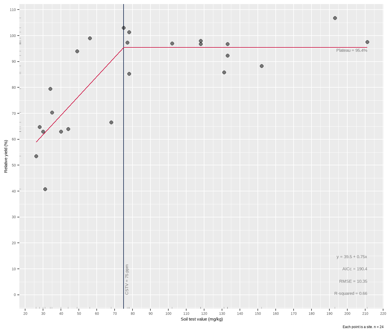
The critical soil test value for potassium appears to be around 75 mg kg-1 K, lower than with a quadratic plateau model. There are gaps in the data, including a hole between 40-80 ppm STK and 65-90% RY. Basically the model lacks confidence in the fit approaching the join point, and this is reflected in the wide gray RY confidence band shown around the red line in the plot. The experimenter needs more data in that gap.
Now, what if the two points with “high” STK (> 180 ppm), were removed? How would that change the analysis? Go back and test yourself8. How do other models compare? Quadratic plateau? Mitscherlich? Cate-Nelson?
8 Hint: filter()
More resources about nonlinear functions in R
nlraapackage by Fernando Miguez (highly recommend)- he also has a series of YouTube videos worth checking out.
rcompanionpackage - many examples of models also applicable to agronomynlstoolspackageeasynlspackage - it’s quick and dirty, but not as useful as it could benls.multstartpackage - tries lots of starting values to try and better get at the best values for the equation. But I think for LP models,nlraapackage works just fine and using multiple starting values is unnecessary.
Bonus: Quick figure with LP line
What if you just want a quick figure of an LP fitted to your scatter plot points, and do not care so much about the model results and information, etc? Using the self-starting function from nlraa, try the following:
cotton %>%
  ggplot(aes(x, y)) +
  geom_point(size = 2,
             alpha = 0.5) +
  geom_line(stat="smooth",
            method = "nlsLM",
            formula = y ~ SSlinp(x, a, b, jp),
            se = FALSE,
            color = "#CC0000") +
  labs(title = paste(
    "Soil test correlation with linear plateau for", nrow(cotton), "cotton trials"),
    y = "Relative yield (%)",
    x = "Soil Test K (mg/kg)")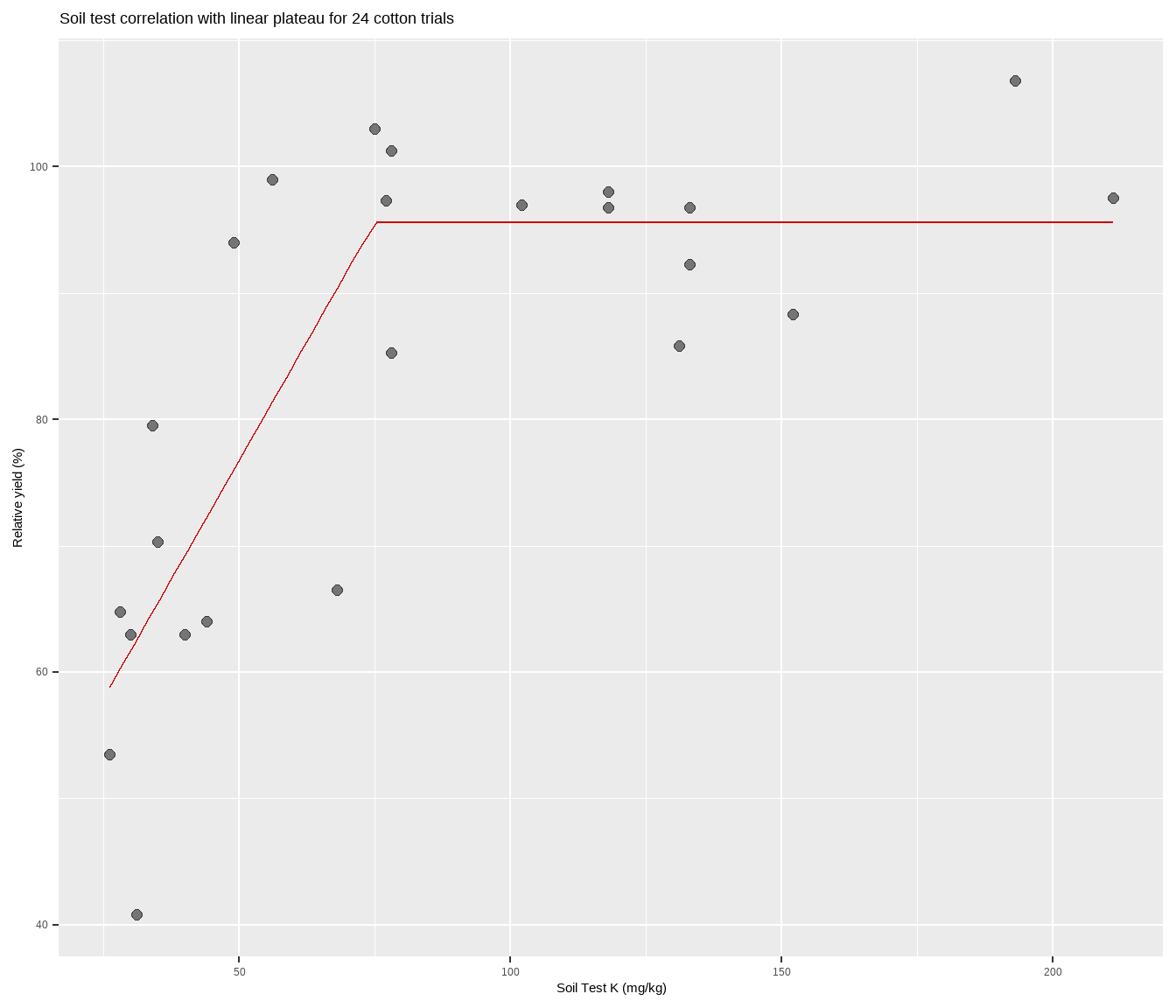
Congratulations! You are now certified to lin-plat in R.